Secret LLM chickens II: Tuning the chicken

When working with an LLM, sometimes it doesn't generate responses in the way you want. Maybe it's being too creative and weird when tasked with serious prompts ("Write me a cover letter for a programming job" "I am a coding wizard and I always min-max my character!"), or it's being too serious when you want to do some creative writing ("Write me a story" "You are tired and you lie down and go to sleep. The end."). This can be tweaked by making certain adjustments to the sampling mechanism—aka "the chicken."

This blog post continues from my previous article, The secret chickens that run LLMs, and you should read that first to understand what a "stochastic chicken" is.

---

Generated with OpenAI DALL-E 3 and edited by the author.

Some key points I'll address here are:

• The "chicken" can be tuned, using inference hyperparameters like temperature, top-k, and top-p. These serve as dials to fine-tune the randomness introduced by the stochastic process, balancing creativity and coherence in the text they generate.
• Adjusting the temperature parameter can make the model's outputs more predictable and less random at lower values, or more diverse and less deterministic at higher values.
• Modifying the top-k and top-p parameters fine-tunes the sampling process by limiting the set of possible next words.
• Top-k restricts the model to choose from the $k$ most likely next words, while top-p uses a probability threshold to create a dynamic set of options. These tweaks help balance creativity with coherence, allowing the LLM to better meet specific needs or experimental conditions.
• Even when using top-k, the astronomical number of possible text sequences challenges the idea of detecting originality and plagiarism. It's nearly impossible to prove the source of any specific piece of text generated by these models, although LLM-generated text can be recognizable due to the language and style used.

note

As in my previous "secret chickens" post, I frequently use the term word instead of token to describe what an LLM predicts. This is just a useful simplification to avoid having to address why the model might predict half a word or a semicolon, since the underlying principles of the "stochastic chicken" are the same.

If you've ever dug into the optional tuning knobs of an LLM provider API, you might have references to tuning "inference hyperparameters" to control how "creative" an LLM can be. These are ways of finding a balance between coherence (sticking to a topic or narrative) and creativity (introducing novel ideas or phrases).

What's a hyperparameter?

When training a neural network, a hyperparameter is a value used to control the learning process and is set before training a model, as opposed to the parameters which are learned during training (and are part of the model itself). Hyperparameters influence various aspects of training including the structure of the neural network (like the number of layers and the number of units per layer), as well as how the network is trained (like the learning rate, batch size, and the number of epochs). These last three explained in simplified terms are:

• Learning rate: How fast the model learns. If the model goes too slowly, it might not learn properly, and if it goes too fast it might skip right over what it needs to learn.
• Number of epochs: How long the model learns. The total number of times the algorithm will work through training data (going through all the data one time is a single epoch).
• Batch size: How many things the model learns at the same time. This is often a trade-off based on how much compute and memory you have.

---

Study study study!
Generated with OpenAI DALL-E 3 and edited by the author.

What's an inference hyperparameter?

An "inference hyperparameter" refers to a configuration for how a model, particularly language models, produce predictions. These settings are used after training by the end users. The most common ones used are temperature, top-k, and top-p, which control the behavior of the model when generating text. They influence aspects like diversity, randomness, and the overall style of the output. Unlike traditional hyperparameters set prior to training to guide the learning process, inference hyperparameters are set to optimize performance for specific tasks when actually using the model.

What may come as a surprise is that these inference hyperparameters don't modify the massive underlying neural network part of these models at all.

They affect the chicken.

---

An unbalanced chicken finding the optimal tuning
Generated with Midjourney 6 and edited by the author

tip

Hyperparameters are set when training a model, and inference hyperparameters are set when using a trained model.

Common inference parameters

Let's take a closer look at these "chicken tuning" mechanisms.

Temperature

Temperature is an inference hyperparameter used to control the randomness of predictions by scaling the logits (the raw output scores from the model) before applying the softmax function to get probabilities. The temperature parameter basically adjusts how conservative or adventurous the model's predictions are.

Temperature = 1

When the temperature is set to 1, it has no effect on the logits, and the model produces outcomes based on the trained probabilities. This is the default setting, where no scaling is applied, and the chicken's choices won't be affected.

---

The original stochastic chicken making a choice
Chicken and feed generated with OpenAI DALL-E 3 and edited by the author.

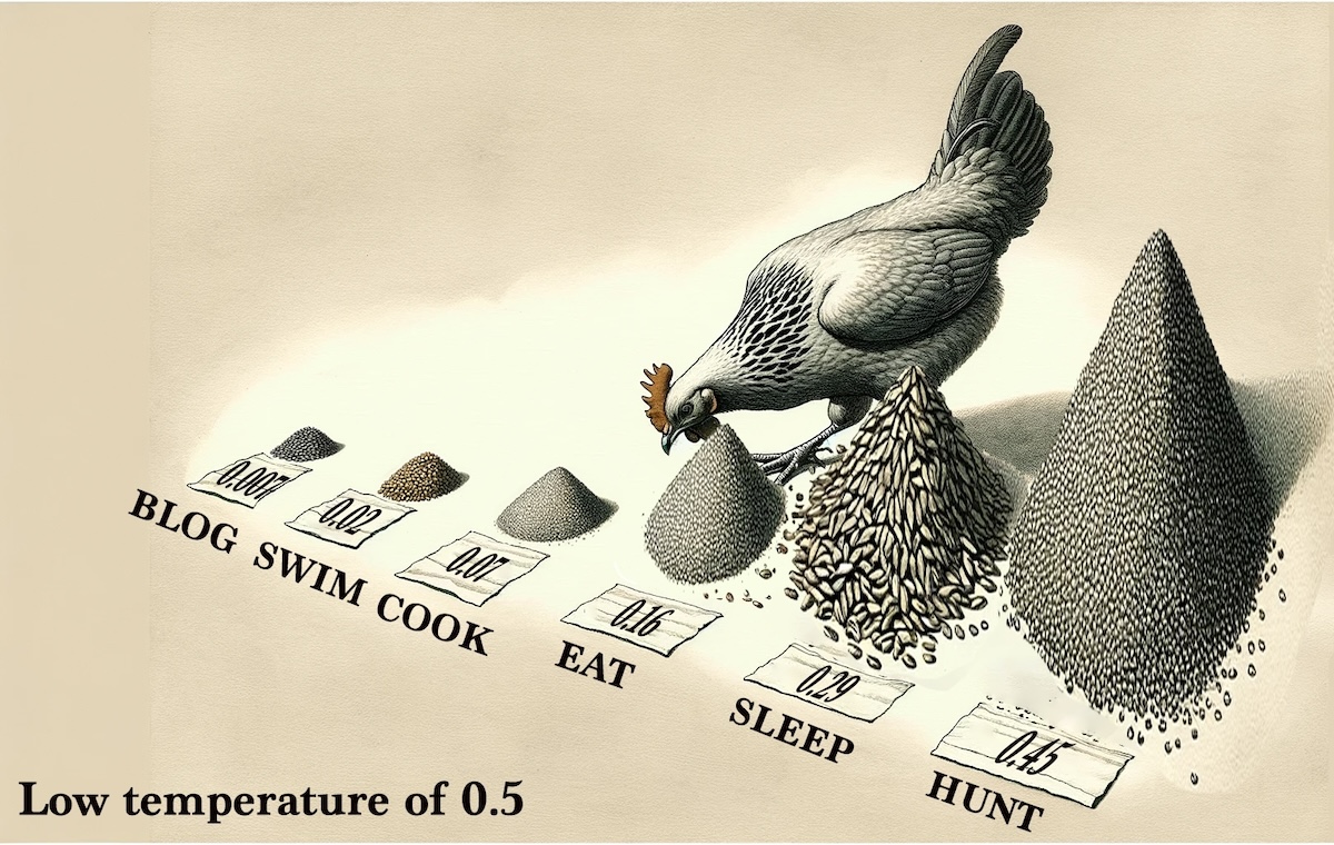
Temperature < 1 (e.g., 0.5)

Lowering the temperature makes the model more confident in its outputs by increasing the gap between the probability of the most likely outcomes and the rest. This makes the chicken's choices less diverse and more deterministic; how could any chicken ignore that huge pile by the word "hunt"? A lower temperature is useful when you want the model to take fewer risks and stick closely to the most likely predictions. This can, however, lead to a lack of variety and potentially more repetitive outputs since, as the temperature approaches $0$, it approximates greedy decoding (with all the problems previously discussed).

---

Using a lower temperature of 0.5, the differences between the probabilities have increased
Chicken and feed generated with OpenAI DALL-E 3 and edited by the author.

Example of generating text with low temperature

Tell me a story about a cat.

Once upon a time, in a cozy little house on the edge of town, lived a cat named Whiskers. Whiskers was a fluffy, grey tabby who loved nothing more than lounging in the sunbeams that danced through the living room windows. Each day, Whiskers would embark on a small adventure in the backyard, chasing butterflies and exploring the garden. In the evenings, Whiskers would curl up on the lap of their owner, purring contentedly as they were petted. Life was simple and serene for Whiskers, the beloved cat.

How is low temperature calculated?

Math & Python code (optional technical content)

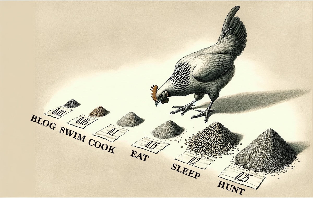
Using our original distribution with probabilities of 0.03, 0.05, 0.1, 0.15, 0.2, and 0.25. How would these change if we used a temperature of 0.5?

Given a distribution of probabilities $P = [0.03, 0.05, 0.1, 0.15, 0.2, 0.25]$ and a temperature $T = 0.5$, we adjust the probabilities as follows:

1. Compute the logits: In this context, you can think of logits as the pre-softmax outputs that the model uses to calculate probabilities. However, since we start with probabilities and want to adjust them by temperature, we reverse-engineer logits by taking the natural logarithm of the probabilities. Thus, the logit for each probability $p_i$ in $P$ is given by:

   $$\text{logit}(p_i) = \log(p_i)$$

2. Scale the logits by the temperature: We then scale these logits by dividing them by the temperature $T$. This step adjusts the distribution of the logits based on the temperature value. For a temperature of $0.5$, the scaling is:

   $$\text{scaled\_logit}(p_i) = \frac{\log(p_i)}{T}$$

3. Convert the scaled logits back to probabilities: We use the softmax function to convert the scaled logits back into probabilities. The softmax function is applied to the scaled logits, ensuring that the output probabilities sum to $1$. The softmax of a scaled logit $s_i$ is given by:

   $$\text{softmax}(s_i) = \frac{e^{s_i}}{\sum_j e^{s_j}}$$

   where $s_i$ is the scaled logit for probability $p_i$, and the denominator is the sum of the exponential of all scaled logits in the distribution. This ensures that the adjusted probabilities sum to $1$.

Putting it all together for each probability $p_i$ in $P$ and a temperature $T = 0.5$, the adjusted probability $p_i'$ is calculated as:

$$p_i' = \frac{e^{\frac{\log(p_i)}{0.5}}}{\sum_j e^{\frac{\log(p_j)}{0.5}}}$$

This formula shows how each original probability is transformed under the influence of the temperature. By applying this process to our original probabilities with $T = 0.5$, we enhance the differences between them, making the distribution more "peaky" towards higher probabilities, as seen with the new probabilities approximately becoming 0.007, 0.018, 0.072, 0.163, 0.289, and 0.452.

note

Step 1 is likely not necessary in practice, since the model's outputs would likely be logits, and thus transforming probabilities back into logits isn't needed. However, since we started with probabilities for illustrative purposes, we transformed them to logits in the example.

Python code for calculating probabiltities with temperature 0.5

import numpy as np
# Original probabilities
probabilities = np.array([0.03, 0.05, 0.1, 0.15, 0.2, 0.25])

# Temperature
temperature = 0.5

# Adjusting probabilities with temperature
adjusted_probabilities = np.exp(np.log(probabilities) / temperature)
adjusted_probabilities /= adjusted_probabilities.sum()

adjusted_probabilities

Output

array([0.00650289, 0.01806358, 0.07225434, 0.16257225, 0.28901734,
       0.4515896 ])

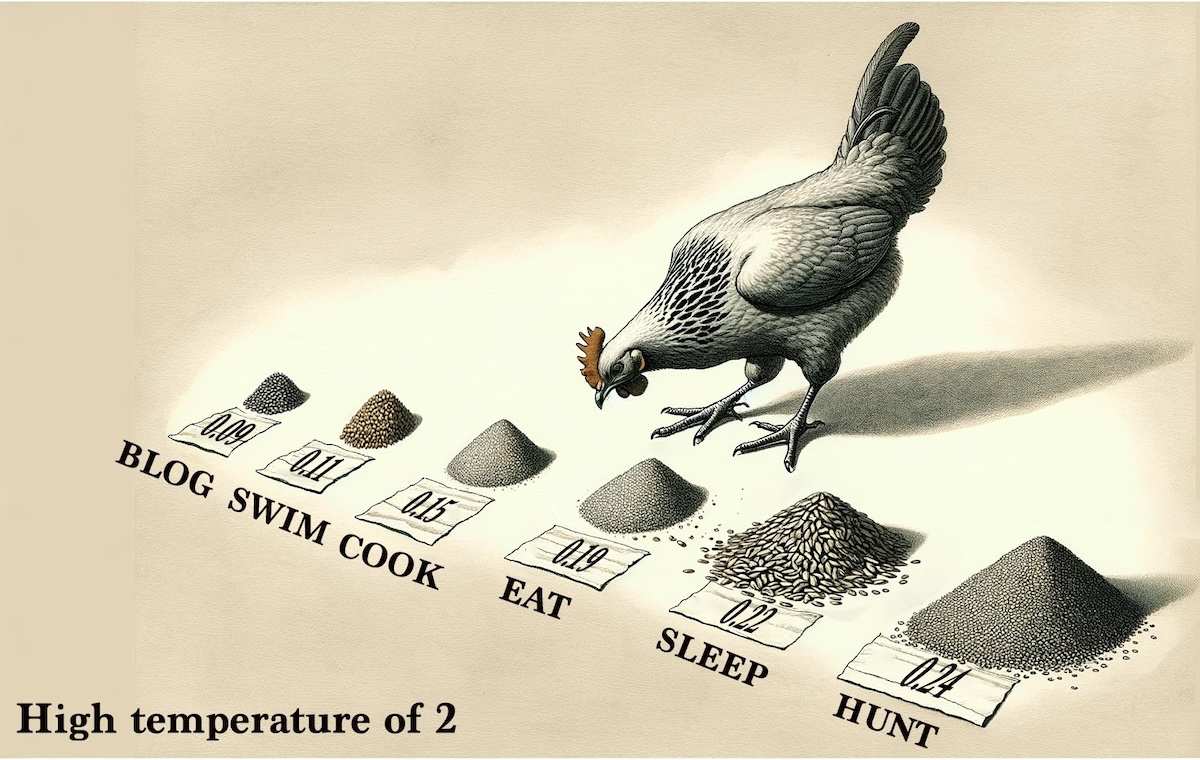
Temperature > 1 (e.g., 2)

Increasing the temperature makes the model's predictions more uniform by reducing the differences between the logits. In the below image, while the highest probability of $0.24$ has only been reduced slightly, the lowest probability of $0.03$ has tripled to $0.09$. This means all the words in the vocabulary now have a more equal chance of being chosen by the chicken. This leads to higher randomness in the output, allowing for more diverse and sometimes more creative or unexpected predictions; a higher temperature is useful when you want the model to explore less likely options or when generating more varied and interesting content. However, too high a temperature might result in nonsensical or highly unpredictable outputs, because the model will start considering very low probability words that make no refrigerator.

---

Using a higher temperature of 2, the differences between the highest and lowest probabilities have decreased
Chicken and feed generated with OpenAI DALL-E 3 and edited by the author.

Example of generating text with high temperature

Tell me a story about a cat.

In the neon-lit streets of Neo-Tokyo, a cybernetic cat named Z3-R0 roamed, its AI brain whirring with thoughts. Tasked with the mission of uncovering a hidden data drive that could save the city from imminent doom, Z3-R0 leaped from rooftop to rooftop, its metallic tail flickering with electric sparks. Along the way, Z3-R0 encountered a gang of robo-rats plotting their own scheme. Using its laser claws and quick wits, Z3-R0 outmaneuvered the rats, secured the data drive, and raced against the clock to deliver it to the rebel base. In the end, Z3-R0 wasn't just a cat; it was a hero of the digital night.

How is high temperature calculated?

Math & Python code (optional technical content)

Using our original distribution with probabilities of 0.03, 0.05, 0.1, 0.15, 0.2, and 0.25. How would these change if we used a temperature of 0.5?

Given a distribution of probabilities $P = [0.03, 0.05, 0.1, 0.15, 0.2, 0.25]$ and a temperature $T = 2$, we adjust the probabilities as follows:

1. Compute the logits: In this context, you can think of logits as the pre-softmax outputs that the model uses to calculate probabilities. However, since we start with probabilities and want to adjust them by temperature, we reverse-engineer logits by taking the natural logarithm of the probabilities. Thus, the logit for each probability $p_i$ in $P$ is given by:

   $$\text{logit}(p_i) = \log(p_i)$$

2. Scale the logits by the temperature: We then scale these logits by dividing them by the temperature $T$. This step adjusts the distribution of the logits based on the temperature value. For a temperature of $2$, the scaling is:

   $$\text{scaled\_logit}(p_i) = \frac{\log(p_i)}{T}$$

3. Convert the scaled logits back to probabilities: We use the softmax function to convert the scaled logits back into probabilities. The softmax function is applied to the scaled logits, ensuring that the output probabilities sum to $1$. The softmax of a scaled logit $s_i$ is given by:

   $$\text{softmax}(s_i) = \frac{e^{s_i}}{\sum_j e^{s_j}}$$

   where $s_i$ is the scaled logit for probability $p_i$, and the denominator is the sum of the exponential of all scaled logits in the distribution. This ensures that the adjusted probabilities sum to $1$.

Putting it all together for each probability $p_i$ in $P$ and a temperature $T = 2$, the adjusted probability $p_i'$ is calculated as:

$$p_i' = \frac{e^{\frac{\log(p_i)}{2}}}{\sum_j e^{\frac{\log(p_j)}{2}}}$$

This formula demonstrates how we adjust each probability with the temperature. Applying this method to our original set of probabilities with $T = 2$ results in a flatter distribution. The differences between probabilities are reduced, making the distribution more uniform and reducing the variance in outcomes, as seen with the new probabilities approximately becoming 0.085, 0.109, 0.154, 0.189, 0.218, and 0.244.

note

Step 1 is likely not necessary in practice, since the model's outputs would likely be logits, and thus transforming probabilities back into logits isn't needed. However, since we started with probabilities for illustrative purposes, we transformed them to logits in the example.

Python code for calculating probabilities with temperature 2

import numpy as np
# Original probabilities
probabilities = np.array([0.03, 0.05, 0.1, 0.15, 0.2, 0.25])

# Temperature
temperature = 2

# Adjusting probabilities with temperature
adjusted_probabilities = np.exp(np.log(probabilities) / temperature)
adjusted_probabilities /= adjusted_probabilities.sum()

adjusted_probabilities

Output

array([0.08459132, 0.10920692, 0.15444191, 0.18915193, 0.21841384,
       0.24419409])

Practical Application

Adjusting the temperature allows users of language models to balance between predictability and diversity in the generated text. For instance, in creative writing or brainstorming tools, a slightly higher temperature might be preferred to inspire novel ideas or suggestions. Conversely, for applications requiring high accuracy and relevance, such as summarization or technical writing, a lower temperature might be more appropriate.

info

If you've used OpenAI's API, you might note that they use a temperature parameter ranging from 0 to 1, which is inconsistent with conventional temperature in language models. It's likely that they're mapping this 0 to 1 range to a broader, internally defined temperature scale while managing the complexity of a temperature-based chicken in the background.

---

Top-k

Another method of "tuning the chicken" is called top-k sampling. The "k" in top-k stands for a specific number that restricts the selection pool to the top "k" most likely next words according to the model's predictions. Again, the primary goal of top-k sampling is to strike a balance between randomness and determinism in text generation.

How top-k works

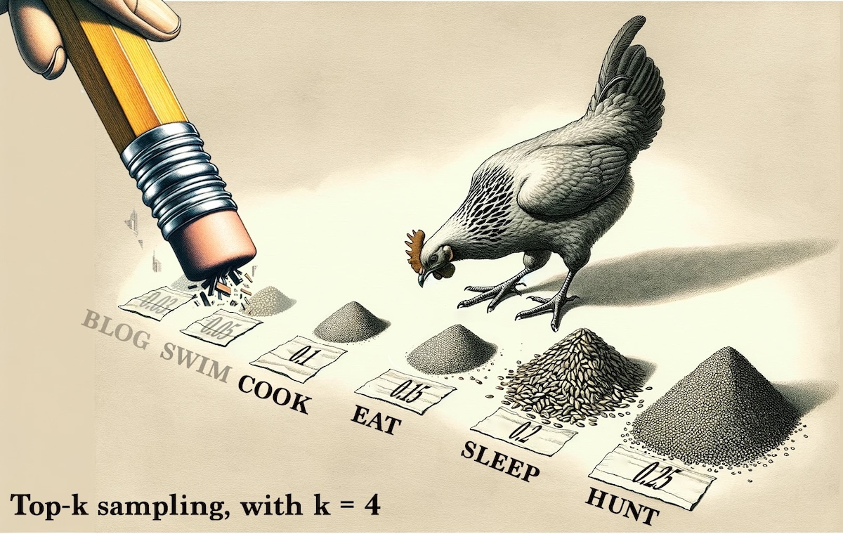
1. Prediction: At each step in the text generation process, the model predicts a probability distribution over the entire vocabulary for the next word, based on the context of the words generated so far.
2. Selection of Top-k Words: From this distribution, only the top "k" words with the highest probabilities are considered for selection. This subset represents the most likely next word according to the model.

---

With a top-k of 4, we need to remove all words other than the top 4 options.
Chicken and feed generated with OpenAI DALL-E 3 and edited by the author.

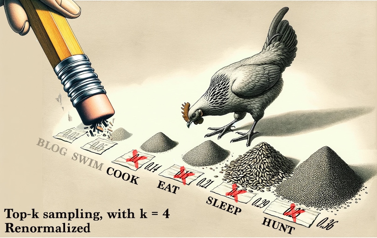
3. Renormalization: The probabilities of these top "k" words are then renormalized so that they sum up to 1. This step ensures that one of these words can be selected based on their relative probabilities within this restricted set. Note that the 4 piles still being considered have grown in size.

---

We now renormalize so that the probabilities add up to 1
Chicken and feed generated with OpenAI DALL-E 3 and edited by the author.

4. Sampling: The chicken finally chooses the following word from this renormalized subset of top "k" words. This introduces variability in the generation process, allowing for diverse and potentially more creative outputs.

Before and after top-k with $(k=4)$

Activity	blog	meditate	cook	eat	sleep	hunt
Original Probability	0.03	0.05	0.1	0.15	0.2	0.25
Top-k $(k=4)$ Probability	0.00	0.00	0.14	0.21	0.29	0.36

note

Remember, this is a heavily simplified example. In reality, the original values would contain many more probabilities, 50,257 in the case of GPT-3. Top-k with $k=4$ would have a large impact on the chicken.

How is top-k calculated?

Math & Python code (optional technical content)

Here's how to compute top-k sampling with $k = 4$ on the set of probabilities

$$P = [0.03, 0.05, 0.1, 0.15, 0.2, 0.25] \text{ with } k = 4:$$

1. Sort the probabilities in descending order: This step isn't necessary for this example, since the probabilities are already sorted, but it's necessary to ensure that we can select the top 4 probabilities.

2. Select the top $k$ probabilities: We choose the four highest probabilities from $P$. Given our $P$, the top 4 probabilities are $0.25$, $0.2$, $0.15$, and $0.1$.

3. Renormalize the selected probabilities: To ensure that these top $k$ probabilities sum to $1$, we renormalize them. The renormalized probability for each selected outcome $p_i$ is calculated as:

   $p_i' = \frac{p_i}{\sum_{j=1}^{k} p_j}$

   where $\sum_{j=1}^{k} p_j$ is the sum of the top $k$ probabilities, ensuring they sum to $1$.

4. Sampling: Finally, we let the chicken choose randomly from these top $k$ adjusted probabilities.

For our given probabilities and $k = 4$, the top 4 probabilities are $0.1$, $0.15$, $0.2$, and $0.25$, which sum to $0.7$. Renormalizing gives us:

$$p_i' = \frac{p_i}{0.7}$$

for each of the top 4 probabilities. This focuses the sampling on the most likely outcomes and leaves out the least likely ones. This guides the generation toward more likely (and maybe even more logical) continuations while still allowing for some randomness and variation. We get the new renormalized top-4 probabilities of 0.14, 0.21, 0.29, and 0.36, which add up to 1.0.

note

Step 1 is likely not necessary in practice, since the model's outputs would likely be logits, and thus transforming probabilities back into logits isn't needed. However, since we started with probabilities for illustrative purposes, we transformed them to logits in the example.

Python code for calculating probabilities top-k with k = 4

import numpy as np

# Original probabilities
probabilities = np.array([0.03, 0.05, 0.1, 0.15, 0.2, 0.25])

# Setting k = 4
k = 4

# Step 1: Select the top-k probabilities
top_k_probabilities = np.sort(probabilities)[-k:]

# Step 2: Renormalize the selected probabilities so they sum to 1
renormalized_top_k_probs = top_k_probabilities / top_k_probabilities.sum()

print("Top-k Probabilities:", top_k_probabilities)
print("Renormalized Top-k:", renormalized_top_k_probs)

Output

Top-k Probabilities: [0.1  0.15 0.2  0.25]
Renormalized Top-k: [0.14285714 0.21428571 0.28571429 0.35714286]

Practical Application

Adjusting the value of "k" allows for tuning the balance between randomness and determinism. A small top-k value restricts the model to choose the next word from a smaller set of the most probable words, leading to more predictable and safer outputs. A large top-k value allows for a wider selection of words, increasing the potential for creativity and unpredictability in the text.

Let's look at two examples of how top-k might affect text generation.

Small top-k (e.g., 5): This setting forces the model to pick from a narrower set of options, likely leading to a more conventional and expected description:

Write a futuristic description of a city.

The city of tomorrow gleams under the starlit sky, its skyscrapers adorned with glowing neon lights. Solar panels cover every rooftop, harnessing the power of the sun to fuel the bustling metropolis below. Hovercars zip through the air, following invisible lanes that weave between the buildings. People walk along clean, green sidewalks, their steps powered by energy-generating tiles. This is a place of harmony, where technology and nature coexist in a sustainable balance, creating a utopia for all who dwell within.

Large top-k (e.g., 50): With this setting, the model has a wider array of words to choose from for each step, potentially leading to a more unique or unconventional description:

Write a futuristic description of a city.

In the heart of the neon jungle, the city thrives, a labyrinth of crystalline towers and levitating gardens. Quantum bridges arc over the meandering rivers of pure light, connecting floating districts that defy gravity with their whimsical architecture. Holographic fauna roam the parks, blending with the urban dwellers who don their digital skins as easily as clothes. Here, the air vibrates with the hum of anti-gravitational engines, and the night sky is a canvas for the aurora technicolor, a testament to the city's fusion of art and science. Cybernetic street performers and AI poets share tales of other dimensions, inviting onlookers to imagine worlds beyond their wildest dreams.

As you can see, a smaller top-k tends to produce more grounded and straightforward descriptions, while a larger top-k opens the door to more inventive and sometimes surreal narratives.

tip

Top-k with $k=1$ is equivalent to greedy decoding.

---

Top-p (nucleus sampling)

Top-p sampling, also known as nucleus sampling, offers an alternative to top-k sampling and aims to dynamically select the number of words to consider for the next word in a sequence, based on a cumulative probability threshold $p$. This method allows for more flexibility and adaptability in text generation, as it doesn't fix the number of tokens to sample from, but rather adjusts this number based on the distribution of probabilities at each step. The term "nucleus sampling" comes from the method's approach to focusing on a "nucleus" of probable words at each step in the generation process.

How top-p sampling works

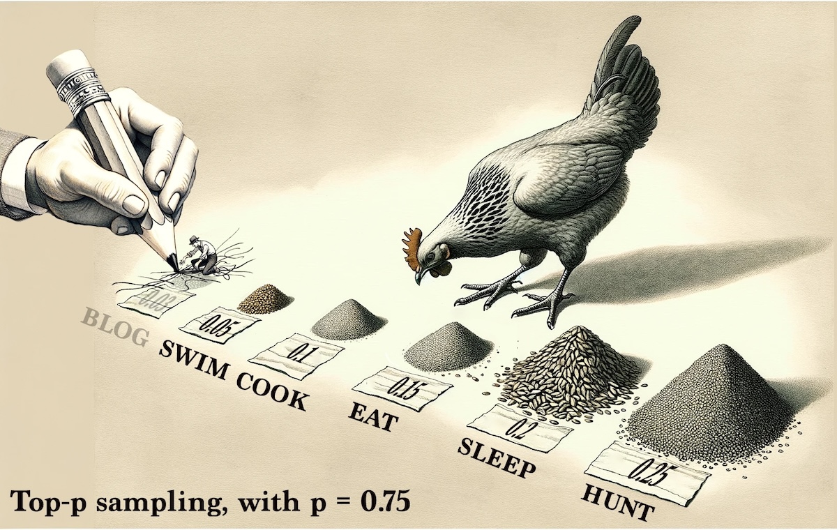
1. Probability Distribution: Given a probability distribution for the next word predicted by a language model, sort the probabilities in descending order.

2. Cumulative Probability: Calculate the cumulative sum of these sorted probabilities.

3. Thresholding: Select the smallest set of words whose cumulative probability exceeds the threshold $p$. This threshold $p$ is a hyperparameter, typically set between 0.9 and 1.0, which determines how much of the probability mass to include in the sampling pool. In our example, since we're only showing the top 6 words, I'm using $p=0.75$ to eliminate only the smallest probability.

---

With a top-p of 0.75, we need to remove all words other than the top 5 options.
Chicken and feed generated with OpenAI DALL-E 3 and edited by the author.

4. Renormalize: The selected probabilities are then renormalized to sum to 1.

---

With a top-p of 0.75, we need to remove all words other than the top 5 options.
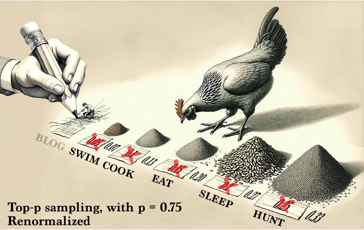
Chicken and feed generated with OpenAI DALL-E 3 and edited by the author.

5. Sampling: Finally, the chicken chooses the next word from this renormalized subset.

Before and after top-p with $(p=0.75)$

Activity	blog	meditate	cook	eat	sleep	hunt
Original Probability	0.03	0.05	0.1	0.15	0.2	0.25
Top-p $(p=0.75)$ Probability	0.00	0.07	0.13	0.20	0.27	0.33

note

As with top-k, remember that this is a heavily simplified example. In reality, the original values would contain many more probabilities, 50,257 in the case of GPT-3. Top-p with $p=0.75$ would have a large impact on the chicken.

How is top-p calculated?

Math & Python code (optional technical content)

Using top-p (nucleus) sampling with a cumulative probability threshold of $p = 0.75$ on the set of probabilities

$$P = [0.03, 0.05, 0.1, 0.15, 0.2, 0.25]$$

involves selecting the smallest set of the most probable outcomes whose cumulative probability exceeds the threshold.

1. Sort Probabilities: First, sort the probabilities in descending order to prioritize higher probabilities. For $P$, when sorted, we have $[0.25, 0.2, 0.15, 0.1, 0.05, 0.03]$.

2. Cumulative Sum: Calculate the cumulative sum of these sorted probabilities. The cumulative sums of the sorted $P$ are approximately $[0.25, 0.45, 0.6, 0.7, 0.75, 0.78]$.

3. Apply the Threshold $p = 0.75$: Identify the smallest set of probabilities whose cumulative sum exceeds $0.75$. In our case, when we reach $0.05$ in the sorted list (cumulative sum $= 0.75$), we've exceeded the threshold $p$.

4. Selected Subset: Based on the threshold, we select the probabilities $[0.25, 0.2, 0.15, 0.1, 0.05]$. Notice that the cumulative probability of these selected probabilities is $0.75$, which meets our threshold condition.

5. Renormalize Probabilities: The selected probabilities are then renormalized so they sum up to 1, to be used for sampling. The renormalization is calculated as follows:

   $$p_i' = \frac{p_i}{\sum_{j=1}^{n} p_j}$$

   where $\sum_{j=1}^{n} p_j = 0.75$ for the selected probabilities, and $p_i$ represents each selected probability.

6. Sampling: Finally, let the chicken choose the next word from this renormalized subset according to the adjusted probabilities.

Description

In top-p sampling with $p = 0.75$, we dynamically adjust the size of the set from which we sample based on the cumulative probability threshold. Unlike a fixed-size set in top-k sampling, the size of the set in top-p sampling can vary depending on the distribution of the probabilities. In this example, by setting $p = 0.75$, we focus on a subset of outcomes that collectively represent the most probable $75\%$ of the distribution. This method means that we're sampling from outcomes that are collectively likely while still allowing for variability and surprise in the generated sequence.

Python code for calculating probabilities top-p with p = 0.75

import numpy as np

# Original probabilities
probabilities = np.array([0.03, 0.05, 0.1, 0.15, 0.2, 0.25])

# Setting the cumulative probability threshold for top-p sampling
p = 0.75

# Sort the probabilities in descending order
sorted_probabilities = np.sort(probabilities)[::-1]

# Calculate the cumulative sum of the sorted probabilities
cumulative_sums = np.cumsum(sorted_probabilities)

# Find the index where the cumulative sum just exceeds or meets p=0.75,
# and select up to that index. This ensures we include probabilities 
# up to the point where the cumulative sum is closest to 0.75
top_p_cutoff_index = np.where(cumulative_sums >= p)[0][0] + 1

# Select the probabilities up to the cutoff index
top_p_probabilities = sorted_probabilities[:top_p_cutoff_index]

# Renormalize the selected probabilities so they sum to 1
renormalized_top_p_probs = top_p_probabilities / np.sum(top_p_probabilities)

print("Top-p Probabilities:", top_p_probabilities)
print("Renormalized Top-p:", renormalized_top_p_probs)

Output

Top-p Probabilities: [0.25 0.2  0.15 0.1  0.05]
Renormalized Top-p: [0.33333333 0.26666667 0.2 0.13333333 0.06666667]

Practical Application

Unlike top-k sampling, which selects a fixed number of tokens $k$, top-p sampling dynamically adjusts the number of tokens based on their probability distribution. Top-p sampling is effective in excluding the long tail of low-probability words without arbitrarily limiting the choice to a fixed number of top probabilities. This can prevent the inclusion of very unlikely words while still allowing for a rich variety of output.

As we did before, let's look at two examples of how top-p might affect text generation.

Small top-p (e.g., 0.5): This setting will likely produce a more straightforward and possibly familiar narrative:

Imagine a world where plants can communicate with humans.

In a world where plants can communicate with humans, gardens and forests become places of deep conversation and learning. Trees share ancient wisdom about the planet's history, while flowers whisper secrets about the medicinal properties of their kin. Humans, in turn, learn to listen to the subtle languages of leaves and roots, developing a symbiotic relationship with the plant kingdom. This newfound communication leads to a harmonious existence, where environmental destruction is halted, and humans work alongside plants to restore the Earth's ecosystems. The air is cleaner, the forests are fuller, and the earth thrives as plants and humans share a mutual understanding and respect.

Large top-p (e.g., 0.9): This setting allows for broader and potentially more imaginative exploration:

Imagine a world where plants can communicate with humans.

In this verdant world, plants do not merely communicate; they are eloquent orators, poets, and philosophers, engaging in intricate dialogues with humans. Through a symphony of scents, colors, and vibrations, they convey not just thoughts, but emotions and artistic expressions. Urban landscapes are transformed into interactive ecosystems where each street corner reveals a new botanical narrative. Walking through parks becomes an immersive experience, as trees recount tales of ecological battles and victories, and flowers critique the quality of urban air with sarcastic wit. Innovative technologies emerge to translate photosynthesis-driven pulses into music, turning forests into concert halls and making agriculture an act of cultural exchange. In this world, plants educate humans about sustainability and creativity, fundamentally altering the fabric of society and fostering an era of unprecedented environmental empathy and artistic flourishing.

These examples show how adjusting the top-p value can influence the directness, creativity, and scope of the generated content.

tip

Top-p with $p=1$ is equivalent to the chicken choosing from all words in the vocabulary.

Even with top-k, there's still no way to definitively prove that a given text was generated

Previously we found that the number of different texts that an LLM can generate is so large that it might as well be infinite. The number we found in that section, $10^9402$, is too large to be useful, so perhaps limiting the vocabulary with top-k or top-p we might make it more reasonable.

First we calculate a more realistic estimate of the number of possible combinations with top-k where $k=40$. We'll use top-k only, since temperature doesn't affect the number of considered tokens, and top-p depends on the probabilities predicted.

We can make some assumptions for a simplified calculation:

1. Vocabulary Size: 50,257 tokens.
2. Sequence Length: 2,000 tokens.
3. Sampling Technique: top-k with $k=40$

Using top-k sampling with an average of 40 choices per token, the logarithm (base 10) of the number of possible combinations for a sequence of 2,000 tokens is approximately $3204$. This means the total number of combinations is roughly $10^{3204}$.

This number, while still incredibly large, is significantly smaller than the $10^{9402}$ we calculated for the full vocabulary without sampling constraints. It shows the reduction in combinatorial complexity due to the smaller choice of tokens with top-k. The difference between this and the unrestricted vocabulary scenario shows the impact of these sampling techniques in making text generation more manageable, and less prone to extreme outliers.

However, it's still such a stupidly large number that it might as well be infinite. The chances of generating 2,000 tokens that have been generated before in the same order are effectively zero. Thus, it isn't possible to show that a generated text was copied from another, and therefore it is impossible to prove plagiarism without a shadow of doubt.

Are there other methods of recognizing generated text? Yes, absolutely, using ways such as the frequency of uncommon words (GPT-4 really loves to say "delve") but that goes beyond the scope of this article.

How is the size of the combinatorial space using top-k calculated?

Math & Python code (optional technical content)

Given a sequence length $N$ and a fixed number of choices per token $K$ in a top-k sampling method, the total number of possible combinations can be estimated. For a top-k of 40 choices per token and a sequence length of 2,000 tokens, the calculation is as follows:

$$\text{Total Combinations} = K^N = 40^{2000}$$

However, to manage the large numbers involved, we calculate the logarithm (base 10) of the total number of combinations. The calculation is given by:

$$\log_{10}(\text{Total Combinations}) = N \cdot \log_{10}(K) = 2000 \cdot \log_{10}(40)$$

Here's how we can calculate this with Python:

Python code for calculating the combinatorial space of a 2,000 token sequence with a top-k of 40

import math

# Top-k sampling
choices_per_token = 40

# Number of tokens in the sequence
sequence_length = 2000

# Calculate the logarithm (base 10) of the number of combinations for top-k sampling methods
log_combinations_top_k = sequence_length * math.log10(choices_per_token)
log_combinations_top_k

Output

3204.1199826559246

Key Takeaways

info

• Hyperparameter Tuning: The article discusses how to tune "stochastic chickens" (sampling mechanisms in LLMs) using inference hyperparameters like temperature, top-k, and top-p. These settings fine-tune the balance between creativity and coherence in generated text.

• Temperature Adjustments: Changing the temperature affects the randomness of model predictions. Lower temperatures result in more deterministic outputs and less diversity, while higher temperatures allow for more random and varied responses.

• Top-k and Top-p Sampling: The top-k parameter limits the model's choices to the k most probable next words, and top-p (nucleus sampling) restricts the choice based on a cumulative probability threshold. These methods refine the model's output by controlling the diversity and predictability of the text.

• Impact on Creativity and Coherence: By adjusting these parameters, users can tailor the model's outputs to be more creative or more focused, depending on the need—whether for creative writing or more factual, straightforward content.

• Uniqueness and Originality: Even with constrained sampling like top-k, the number of possible text sequences remains astronomically high, ensuring that each piece of generated text is nearly always unique.

• Practical Applications: Various settings for these hyperparameters are useful for different scenarios, such as creative writing, technical documentation, or casual dialogue, demonstrating their utility in practical applications.